Machine Learning Final Project
Project maintained by cfletcher33 Hosted on GitHub Pages — Theme by mattgraham
Meet the Team
Group 20
- Carson Fletcher
- Sidney Genrich
- Clemens Koolen
- Andrew Palmer
- Ben Wisehaupt
Motivation
Our project is based on a kaggle competition (LINK) to predict the next price that a US corporate bond might trade at. The movement of asset prices is a highly complex system, making them a key candidate for machine learning techniques. Given the various new platforms on which corporate bonds are traded, and the need for more frequent, up-to-date information of bond prices, we hope to create an algorithm that is able to accurately, and quickly price bonds.
Data
The dataset was provided by the Kaggle competition and consists of microstructure bond trade data. The raw dataset provides a label coumn describing the true trade price, a weight column, 57 features, and 762,678 instances. The weight column is calculated as the square root of the time since the last trade and then scaled so the mean is 1. This weight column is used for evaluation purposes and will be further discussed below. The data structure is easy to work with as there is no time series dependency, and therefore each instance is not dependent on those around it.
The first step of data preprocessing was to clean the data. We first removed irrelevant columns, namely the trade id and reporting delay features. The trade id feature was simply an identifier and had no predictive power. The reporting delay feature was removed because the it was found to be extremely noisy and did not provide any valuable insight. The next step of preprocessing was to remove all rows containing nan, infinite, and missing values. Generally, removing all rows with a corrupted value can be dangerous because it can lead to a severe reduction in the size of your data set. However, after this second step was performed the data consisted of 745,009 instances, so we are confident that this procedure was safe to perfrom and still left us with a significant amount of data to test and train.
Lastly, the data was split into a testing and training set. Because the data does not have any timeseries dependency we were able to use the sklearn test_train_split function to randomly split the data. Because our data set was plentiful we chose to use a split size of 75% training and 25% testing, which resulted in a training size of 558,756 instances and a testing size of 186,253 instances.
Functionality was added to scale the data between zero and one, and normalize the data with a mean of zero and standard deviation of 1. These functions allow us to observe the effectiveness of standardizing the data prior to model implementation and then choose the option that provides the best performance.
Model Implementation
In order to choose our models, we have to first make some observations about our data. The most important observation for our model selection is that unlike many other datasets out there that are composed of seemingly linear data, our data is highly non-linear. This severely limits our scope of machine learning models. As a result, for our supervised learning algorithms, we will be looking at three different levels of decision trees in the form of a simple decision tree, a random forest, and an extreme gradient boosted random forest. We beleive these models will be able to effectively solve our problem because they perform well when using non-linear data. This pivot to new supervised models is the biggest change in our approach from the approach presented in the project proposal.
Principle Component Analysis
Our unsupervised learning model is a principal component analysis which was used to reduce the dimensionality of the data set. Given the complexity of our machine learning models, reducing the number of dimensions is extremely valuable because it reduces the amount of time needed to fit the models.
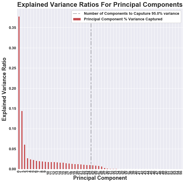
Our principle component analysis was implemented to explain 95% of the variance of the data set. With this parameter the model requires 24 principle components to meet the threshold of required variance. We implemented the PCA using both scaled and normalized data to see how each would affect the final prediction performance . We found that the PCA using normalized data resulted in better performance when the given principle components are used to fit and predict the data.
The plot below highlights the variance explained by each principle component. We can see that a majority of the variance is explained in the first two or three components. This may cause issues when using the principle components to fit and predict as it would put essentially put “all of the eggs” in two or three components.
One large downside of using a PCA is that its only goal is to explain a certain amount of variance. In the process of achieving this goal, the PCA overlooks small differentiations in the data that may provide great predictive power. We will explore the performance of the models when using the principle components to train and test versus when using the original features to train and test.
Decision Tree Regressor
Decision trees are extremely effective at going through a variety of features and splitting on the feature that impacts price the most. They could take long to train, yet are simple to understand and yield great results if your data is not prone to overfitting. One problem we might encounter however, is that we need pretty deep and complicated trees to properly regress our dataset to the accuracy level that we would like. While we could use Decision Trees to give an extremely rough estimate of whether a bond price is going to be higher or lower than what we have seen, our performance evaluation is focused on quantifying the difference in prices.
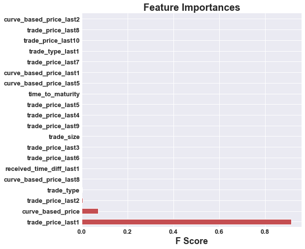
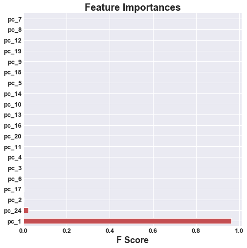
As mentioned before, our effectiveness of decision trees will really come down to the hyperparameter tuning, as a tree too deep, could open us up to overfitting, and a tree too shallow would not split our data enough. Similarly, having too many leaves could overfit our data, while keeping a large variety of bond prices within a leaf could generalize the bond prices too much. We performed a cross validated grid search to optimize the hyperparameters in the table below. The table shows the given hyperparameter and its optimal value.
| Parameter | Without PCA | With PCA |
|---|---|---|
| Splitter | best | random |
| Max Depth | 40 | 45 |
| Max Features | auto | auto |
| Min Samples per Leaf | 4 | 4 |
| Min Samples per Split | 10 | 10 |
| Without PCA | With PCA |
|---|---|
 |
 |
Random Forest Regressor
For our second supervised model, we have chosen a Random Forest Regressor model, as an improvement on our Decision Tree Regressor. Given the complexity of our data, and the complicated process of pricing bonds, we need to attain accuracy on our training data without overfitting, the latter which is common in decision trees. Decision Tree Regressors fail at predicting new data points in a ‘smart’ way as it will just look at previously encountered data points, regardless of bias or specific defining characteristics, and assign a price value to the model. To avoid these problems and still maintain an accurate model with nonlinear data, we will use a random forest. Using the characteristic bootstrapping that a Random Forest employs, we can get rid of bias that might exist in our data. Sample data points will be used to train the trees using a sample of features, after which we will aggregate the results of all of our decision trees that have been trained on different data points and features. The resulting bond price will be more accurate through unbiased data points and features, and aggregated decision tree results. In general, we have taken the benefits of our decision tree, and combined it with unbiased data and smarter prediction.
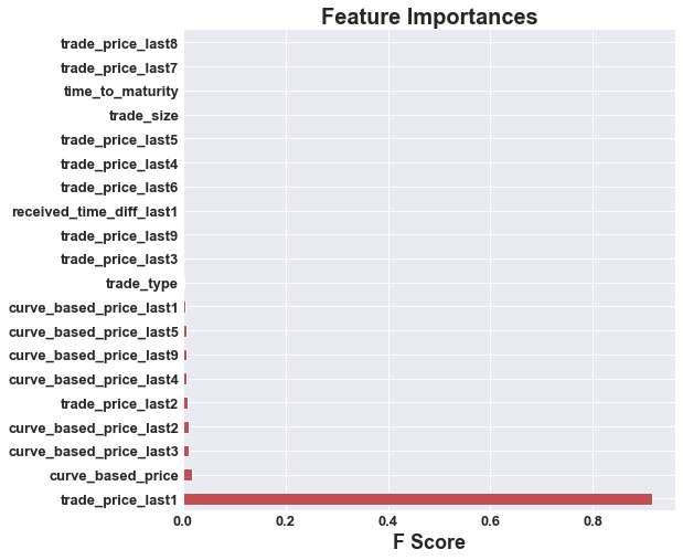
A random forest has two areas of hyperparameter tuning, the forest, and the trees. We will look at both. For example, one of the parameters specific to the random forest is the number of trees, or the max number of features in a bootstrap sample. Oftentimes, the more trees we have the better our model will perform, yet at the cost of speed. Similarly to hyperparameter tuning in decision trees, our previous model, we would want to change hyperparameters in our decision tree, like the maximum number of leaves of a node, or the depth of the tree in order to either improve our accuracy or speed. To implement the parameter tuning, we realized there is a large variability in our data and features. We therefore won’t just run a simple GridSearch with arbitrary hyperparameters as we did in our Decision Tree, as we could either make the model too convoluted, or too simple. Therefore, to give us an idea of what we should put in our cross-validated GridSearch, we will first run a cross-validated RandomSearch, looking at a wide range of hyperparameters and see how it impacts our results. After we have the results of our RandomSearch, we can then run a cross-validated Gridsearch over hyperparameter values closer to our optimal values found in the RandomSearch. Through this, we will get hyperparameters that give us an accurate random forest for our dataset. The table below gives us the hyperparameters and their optimal values.
| Parameter | Without PCA | With PCA |
|---|---|---|
| Max Depth | 45 | 45 |
| Max Features | auto | auto |
| Max Leaf per Node | none | none |
| Min Samples per Leaf | 6 | 6 |
| Min Samples per Split | 10 | 10 |
| Number of Estimators | 10 | 10 |
| Without PCA | With PCA |
|---|---|
 |
 |
Extreme Gradient Boosted Random Forest (XGBoost)
Boosting adds another level of complexity onto our previous methods of Decision Tree Regressor and Random Forest Regressor. In this method our objective function is composed of two parts: (1) a training loss and (2) a regularization term.
More specifically, the tree boosting works as follows:

Which becomes

Where

Practically speaking this is used to optimize one level of the tree at a time using a measurement called Gain. Gain is used to split a leaf into two leaves.

Where lambda is the regularization on the leaf. Interestingly using this Gain is pretty much the same as post pruning, but while building the tree.
A gradient-boosted tree does the above, but with building the tree with respect to the residuals rather than the original data/labels. XGBoost is an implementation of gradient boosting that emphasizes execution speed.
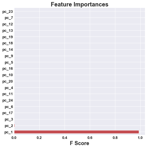
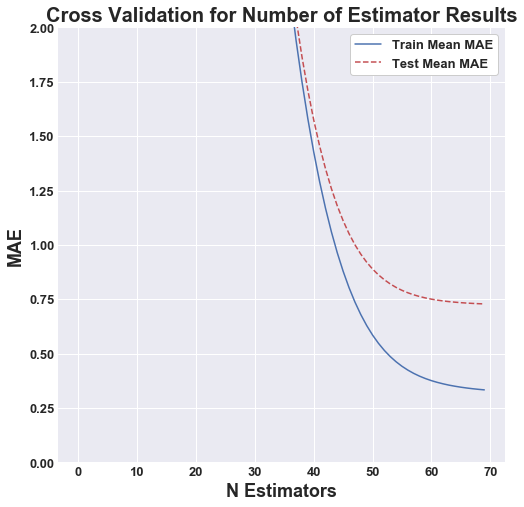
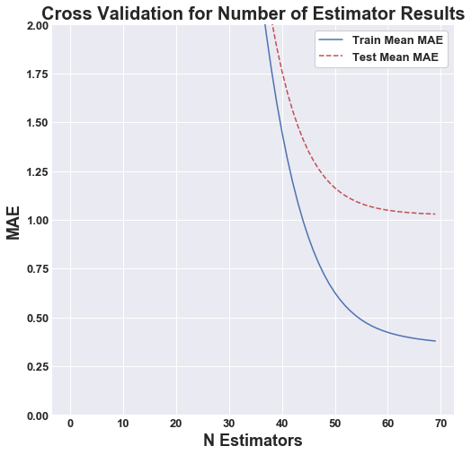
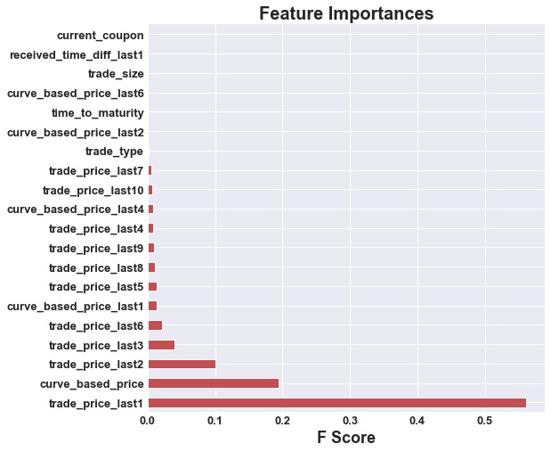
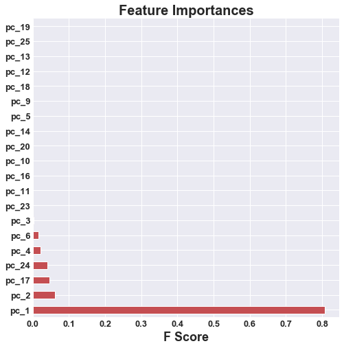
The main hyperparamter for this algorithim is the number of features. This parameter was optimized through cross validation, which is represented by the figures below. We can see as the number of estimators approaches 70, the marginal increase in accuracy begins to faltten. The optimal number of estimators for both secnarios, without PCA and with PCA, was determined to be 70.
| Without PCA | With PCA |
|---|---|
 |
 |
| Without PCA | With PCA |
|---|---|
 |
 |
Performance Evalaution
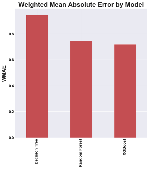
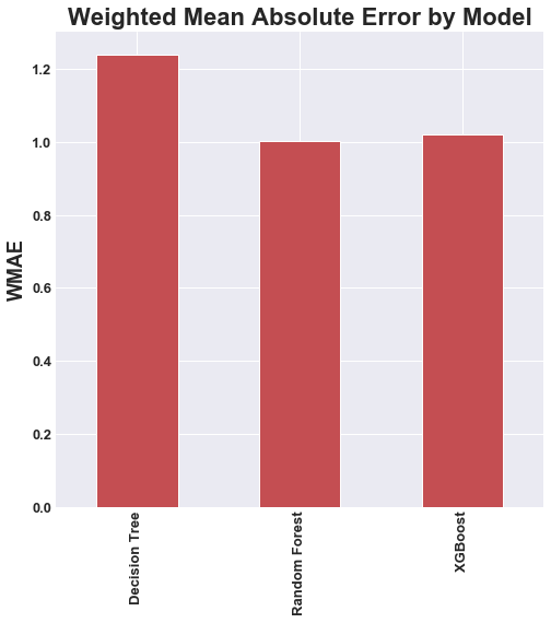
For the Kaggle competition they evaluated performance by calculating the weighted mean absolute error using the weight column mentioned previously. We apply the same method to evaluate our models, and therefore can compare our performance to the competition leaderboard. We can see that the models running without PCA significantly outperformed the models that were running with PCA. This is due to the fact that PCA destroys the slight nuances in the data that have the potential for great predictive power.
Based on our performance below, the Extreme Gradient Boosted Random Forest wihtout PCA was clearly the best model. If we were to enter this model into the Kaggle competition we would have placed in 6th place. The total cash prize for this competition was $17,500.
| Without PCA | With PCA |
|---|---|
 |
 |
| Model | WMAE without PCA | WMAE with PCA |
|---|---|---|
| Decision Tree | 0.9512 | 1.2410 |
| Random Forest | 0.7405 | 1.0038 |
| Extr. Boosted Random Forest | 0.7160 | 1.0212 |
Conclusions
In choosing three increasingly complex tree-based regression models, we were able to demonstrate the increasing predictive power moving from decision tree to random forest to gradient boosted random forest, each performing better than the last. This is what expected moving into the project, as each model was built to corrrect issue with the ones preceeding it. As such, we knew in advance that extreme gradient boosting would take the lead. However, at first, it came as a suprise to us that PCA hindered our performance. After careful thought, we realized that PCA was not the right dimensionality reduction algorithm for the dataset since the feature definitions were diverse and nuanced to the task of pricing bonds. With more time, resources, and computational power, we firmly believe that we could thoroughly tune the hyper-parameters of our model to achieve a significant better prediction accuracy.
Overall, the results we have achieved demonstrate the feasibility of predicting bond prices with a sufficiently complex model, an important task for bond traders around the world. Millions of trades are executed in the bond market on a daily basis. Our best model generated profit of over $96,000 on the test dataset of 186 thousand trades. Scaled up to a commercial level of volume, it is clear that we have succeded in our goal of fortelling the future of bond pricing.